Part 1 / Section 1: Labor and Capital as Aggregate Inputs: Substitutability Section 1.2

The firm's input choice

Even if the firm makes zero profits we can establish how it will optimally choose its inputs. We do this by solving the cost minimization problem. For this, let \(r\) be the rental price of one unit of capital and \(w\) the wage paid for one unit of labor. Suppose that the firm wants to produce \(\overline{Y}\) at the lowest possible cost. Its problem is

\[\begin{equation} \underbrace{C(\overline{Y},r,w)}_{\text{Cost Function}} \;=\; \min_{K,L}\; rK\,+\,wL \qquad\text{subject to}\qquad zF(K,L)\,\geq\, \overline{Y}. \tag{1.4} \end{equation}\]

We can analyze this problem graphically by looking at the properties of the cost and the output constraint. Our graph deals with the choice of capital and labor and so those will be the axes. The cost function is linear in the inputs and so we can graph different levels of cost with what we call an isocost curve:

Definition 1.1: Isocost curve

It is the combinations of capital and labor \((K,L)\) that deliver the same cost level \(\overline{c}\):

\[\begin{align} \overline{c} \;=\; rK \,+\, wL \qquad\longleftrightarrow\qquad K \;=\; \frac{\overline{c}}{r} \,-\, \frac{w}{r}L \;. \tag{1.5} \end{align}\]

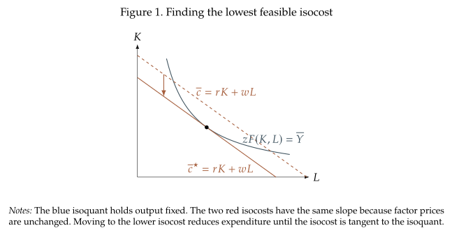
The isocost is a downward-sloping line because increasing either input raises the cost, and so the other input must go down to keep the cost constant. The slope of the isocost tells the rate at which the two inputs must be exchanged to keep the cost constant. That is, the rate at which we can exchange one input for another at market prices. The slope is therefore the relative price, in our case \(w/r\).

The firm's objective is to choose the lowest isocost curve that satisfies the production constraint. That constraint is characterized by an isoquant curve:

Definition 1.2: Isoquant curve

It is the combinations of capital and labor \((K,L)\) that deliver the same output level \(\overline{Y}\):

\[\begin{align} \overline{Y} \;=\; zF\left(K\,,\,L\right)\;. \tag{1.6} \end{align}\]

The isoquant is a downward-sloping curve because increasing either input raises output (reflecting positive marginal products), and so the other input must go down to keep output constant. The shape of the isoquant depends on the properties of the production technology.

The graphical representation of the problem is in Figure 1. The firm will take as given the isoquant and move to lower isocost curves as much as possible.