Part 1 / Section 3: CES Production and Technological Change Overview

Overview

The Cobb--Douglas production function gives us a clean benchmark to study the many issues, but it is too restrictive to study those that depend on the elasticity of substitution. What if capital and labor are easier, or harder, to substitute? We now extend the analysis to a production function that allows for a general elasticity of substitution, but that remains easy to use by imposing that the elasticity of substitution is constant. Accordingly, we call it the constant-elasticity-of-substitution (CES) production function. Extending our analysis to the CES production function will also allow us to study the effects of technological change on the relative factor shares of income as we can now distinguish between technological change geared towards a specific factor (this is the directed technical change that Hicks referred to).

The CES production function is

\[\begin{equation} Y\;=\;z\left( \alpha\left(A_K K\right)^{\frac{\sigma-1}{\sigma}} \;+\;\left(1-\alpha\right)\left(A_L L\right)^{\frac{\sigma-1}{\sigma}} \right)^{\frac{\sigma}{\sigma-1}}, \qquad \sigma>0,\quad \sigma\neq1. \tag{3.1} \end{equation}\]

where \(A_K>0\) and \(A_L>0\) are factor-augmenting technologies. When \(\sigma\,=\,1\) we have the Cobb-Douglas function.

While the function looks more complicated than Cobb--Douglas, it is still easy to use once we realize how to exploit the fact that it has constant returns to scale. The marginal product of capital is

\[\begin{align} \frac{\partial Y}{\partial K} &\;=\; z\frac{\sigma}{\sigma-1} \left( \alpha\left(A_K K\right)^{\frac{\sigma-1}{\sigma}} \;+\;\left(1-\alpha\right)\left(A_L L\right)^{\frac{\sigma-1}{\sigma}} \right)^{\frac{1}{\sigma-1}} \frac{\sigma-1}{\sigma} \alpha A_K^{\frac{\sigma-1}{\sigma}}K^{-\frac{1}{\sigma}}, \tag{3.2} \end{align}\]

We can greatly simplify this expression by noticing that

\[\begin{align} \frac{1}{\sigma-1} \;=\; \left(\frac{\sigma}{\sigma-1}\right)\frac{1}{\sigma}. \tag{3.3} \end{align}\]

The bracket raised to \(\frac{\sigma}{\sigma-1}\) equals \(Y/z\). Keeping the factor \(z\) outside the bracket, we therefore obtain

\[\begin{align} \frac{\partial Y}{\partial K} &\;=\; z \left[\left( \alpha\left(A_K K\right)^{\frac{\sigma-1}{\sigma}} \;+\;\left(1-\alpha\right)\left(A_L L\right)^{\frac{\sigma-1}{\sigma}} \right)^{\frac{\sigma}{\sigma-1}}\right]^{\frac{1}{\sigma}} \alpha A_K^{\frac{\sigma-1}{\sigma}}K^{-\frac{1}{\sigma}}, \tag{3.4} \\ &\;=\; z\left(\frac{Y}{z}\right)^{\frac{1}{\sigma}} \alpha A_K^{\frac{\sigma-1}{\sigma}}K^{-\frac{1}{\sigma}} \nonumber \\ &\;=\; z^{\frac{\sigma-1}{\sigma}}\alpha A_K^{\frac{\sigma-1}{\sigma}}\left(\frac{K}{Y}\right)^{-\frac{1}{\sigma}} . \tag{3.5} \end{align}\]

Similarly, the marginal product of labor is

\[\begin{align} \frac{\partial Y}{\partial L} &\;=\; z^{\frac{\sigma-1}{\sigma}}(1-\alpha) A_L^{\frac{\sigma-1}{\sigma}}\left(\frac{L}{Y}\right)^{-\frac{1}{\sigma}}. \tag{3.6} \end{align}\]

Finally, the MRT is

\[\begin{align} \operatorname{MRT}_{L,K} \;=\; \frac{F_L}{F_K} \;=\; \frac{1-\alpha}{\alpha}\left(\frac{A_L}{A_K}\right)^{\frac{\sigma-1}{\sigma}} \left(\frac{L}{K}\right)^{-\frac{1}{\sigma}}. \tag{3.7} \end{align}\]

We can then get the elasticity of substitution by inverting this equation and applying logarithms:

\[\begin{align} \log\frac{K}{L} \;=\; \sigma\log\frac{\alpha}{1-\alpha} \;+\; \left(\sigma-1\right)\log\frac{A_K}{A_L} \;+\; \sigma\log\operatorname{MRT}_{L,K}. \tag{3.8} \end{align}\]

The elasticity of substitution is therefore constant and equal to \(\sigma\). Three limiting cases help us interpret it. Figure 6 compares their isoquants:

1. \(\boldsymbol{\sigma\,\rightarrow\,\infty}\): The inner and outer exponents both approach one, and the inputs approach perfect substitutes. This gives a linear technology: \(\,Y\;=\;z\left(\alpha A_KK+(1-\alpha)A_LL\right)\).
2. \(\boldsymbol{\sigma\,=\,1}\): The expression in (3.1) is read as a limit and becomes Cobb--Douglas: \(Y\;=\;z(A_KK)^\alpha(A_LL)^{1-\alpha}\). \ In this case we cannot distinguish between factor-augmenting technologies and neutral technological term \(z\) because we can always write \(\widetilde{z}\;=\;z(A_K)^\alpha(A_L)^{1-\alpha}\) and obtain \(Y \;=\;\widetilde{z}K^{\alpha}L^{1-\alpha}\).
3. \(\boldsymbol{\sigma\,\rightarrow\,0}\): The technology approaches a fixed-proportions (or Leontief) technology. Capital and labor become perfect complements: \(Y\;=\;z\min\left\lbrace A_KK,A_LL\right\rbrace\).

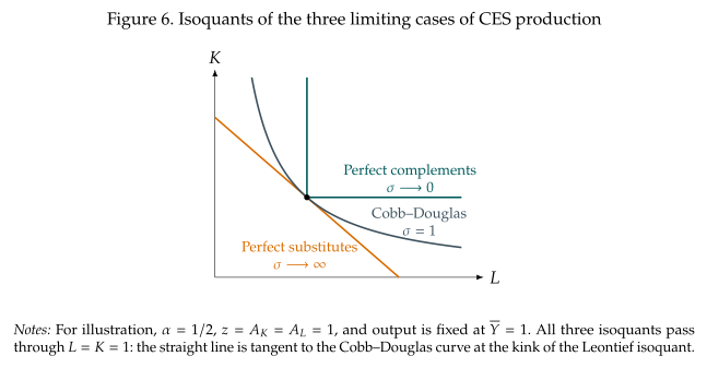
Same as in our general analysis, the elasticity of substitution determines what happens if the relative price of capital and labor changes. At the cost-minimizing input mix, the MRT equals \(w/r\) and

\[\begin{equation} \dd\log(K/L)\;=\;\sigma\,\dd\log(w/r). \tag{3.9} \end{equation}\]

So, if capital becomes cheaper, \(w/r\) rises and the firm chooses a higher \(K/L\). The value of \(\sigma\) tells us by how much. When \(\sigma>1\), the response is stronger than under Cobb--Douglas. When \(\sigma<1\), it is weaker.

Example 3.1: The same price change under two technologies

Suppose \(r\) falls by 10 percent and \(w\) is fixed. If \(\sigma=2\), the firm raises \(K/L\) by approximately 20 percent. If \(\sigma=0.5\), it raises \(K/L\) by only 5 percent. In both cases the firm uses a more capital-intensive technique; the size of the movement differs.

Where does the weird power in the CES come from?

The CES can look daunting because of the many terms it has. But it does not have to be that complicated. We can see why we write the function the way we do by re-deriving our results starting from a simpler function. Consider the following production function:

\[\begin{align} Y\;=\; z\left(\, K^\beta \;+\; L^\beta \,\right)^{\frac{1}{\beta}} \,. \tag{3.10} \end{align}\]

We have dropped the weights and assumed \(A_K=A_L=1\).

The first order conditions give us

\[\begin{align} r &\;=\; pz\left(\cdot\right)^{\frac{1}{\beta}-1} K^{\beta-1} \;=\; pz\left(\cdot\right)^{\frac{1-\beta}{\beta}} K^{\beta-1} \;=\; pz\left(\left(\cdot\right)^{\frac{1}{\beta}}\right)^{1-\beta} K^{\beta-1} \;=\; pz^\beta \left(\frac{K}{Y}\right)^{\beta-1} \tag{3.11} \\ w &\;=\; pz\left(\cdot\right)^{\frac{1}{\beta}-1} L^{\beta-1} \;=\; pz^\beta \left(\frac{L}{Y}\right)^{\beta-1} \tag{3.12} \end{align}\]

So, optimality requires (by taking the ratio of the two equations)

\[\begin{align} \frac{w}{r} \;=\; \text{MRT}_{L,K} \;=\; \left(\frac{L}{K}\right)^{\beta-1} \,. \tag{3.13} \end{align}\]

From this we also get the ratio of income shares:

\[\begin{align} \frac{\alpha_L}{\alpha_K} \;=\; \frac{wL}{rK} \;=\; \left(\frac{L}{K}\right)^{\beta} \,. \tag{3.14} \end{align}\]

Why do we write the power of the CES as \((\sigma-1)/\sigma\) and not just as \(\beta\)?

The reason is that we do not actually care about \(\beta\) directly. Just like in Section 1, we care about the elasticity of substitution:

\[\begin{align} \sigma \;=\; \frac{\partial \log \frac{K}{L}}{\partial \log \frac{w}{r}} \,. \tag{3.15} \end{align}\]

We can figure out the elasticity from the optimality condition:

\[\begin{align} \log \frac{w}{r} \;=\; \left(\beta-1\right) \log \frac{L}{K} \quad \longrightarrow\quad \log \frac{K}{L} \;=\; \frac{1}{1-\beta} \log \frac{w}{r} \,. \tag{3.16} \end{align}\]

From this we see that the elasticity of substitution is

\[\begin{align} \sigma \;=\; \frac{1}{1-\beta} \,. \tag{3.17} \end{align}\]

So, we can replace \(\beta\) in terms of \(\sigma\):

\[\begin{align} \sigma \;=\; \frac{1}{1-\beta} \;\longrightarrow\; 1-\beta \;=\; \frac{1}{\sigma} \;\longrightarrow\; \beta \;=\; 1 - \frac{1}{\sigma} \;\longrightarrow\; \beta \;=\; \frac{\sigma-1}{\sigma} \;. \tag{3.18} \end{align}\]

This gives us the power we use in the CES. Now we can obtain our results directly in terms of the elasticity of substitution without having to translate the level of \(\beta\) into a level of \(\sigma\).