Part 1 / Section 3: CES Production and Technological Change Section 3.1

Factor-augmenting technological change¶

As mentioned above, the CES allows us to study what happens when technology changes in a way that favours a particular factor. An increase in $A_K$ makes every physical unit of capital more effective, while an increase in $A_L$ makes every unit of labor more effective. This is different from increasing $K$ or $L$: it changes what each physical unit can do. It is actually more similar to a change in the price. Being more productive means producing more output with the same physical input, which is (almost) equivalent to having a lower price for that input.

Equation (3.8) lets us separate the price response from the technology response:

\[\begin{equation} \dd\log(K/L) =\sigma\,\dd\log(w/r) +(\sigma-1)\dd\log(A_K/A_L). \tag{3.19} \end{equation}\]

The way in which technology affects the relative demand for inputs depends on the elasticity of substitution. Consider an increase in $A_K$ (or a decrease in $A_L$) with $w/r$ fixed. What happens to the number of physical units of capital relative to labor?

$\boldsymbol{\sigma>1}$: An increase in $A_K$ raises physical $K/L$. The firm finds capital sufficiently easy to substitute toward that the productivity gain increases its relative use.
$\boldsymbol{\sigma=1}$: An increase in $A_K$ does not change physical $K/L$ at fixed prices. This is another special Cobb--Douglas result.
$\boldsymbol{0<\sigma<1}$: An increase in $A_K$ lowers physical $K/L$. Because capital and labor are hard to substitute for each other, each more-effective unit of capital can support the existing labor input with fewer physical units of capital.

The last case is important to understand. When $\sigma<1$, the firm does not value capital less. Effective capital $(A_K K)$ and effective labor $(A_L L)$ are hard enough to substitute that each unit of capital now provides more services, allowing the firm to produce with fewer physical units.

Seeing the technology response in the cost-minimization diagram¶

Figure 7 compares the same increase in capital productivity across the three cases. We hold output, factor prices, and labor productivity fixed, and double $A_K$. For any given amount of labor, doubling $A_K$ halves the capital needed to produce the same output, so the isoquant shifts inward in all cases. The firm can reach the new isoquant with a lower isocost, but the isocost slope $-w/r$ is unchanged because factor prices have not changed. The dots mark the initial and new cost-minimizing bundles (where $\operatorname{MRT}=w/r$).

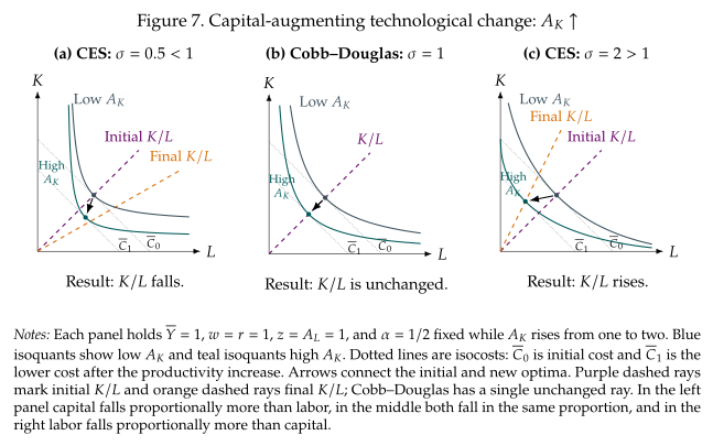
Capital-augmenting technological change: $A_K\uparrow$

To see the change in the input mix, compare the rays from the origin through the two tangency points: the slope of each ray is $K/L$.

With $\sigma<1$, the new ray is flatter: capital falls proportionally more than labor.
With Cobb--Douglas ($\sigma=1$), both points lie on the same ray: the two inputs fall in the same proportion.
With $\sigma>1$, the new ray is steeper: labor falls proportionally more than capital.

The inward shift shows the production-cost saving in all three cases; the change in the ray shows whether the firm also changes its input mix. If we hold production constant this lets the firm produce with fewer inputs (less capital and less labor). If we allow the level of output to adjust we would see that we can now produce more because the lower costs mean lower prices and higher demand. Nevertheless, this higher output will be produced using the new capital to labor ratio $K/L$.