Part 2 / Section 5: Task-Based Model of Production Section 5.4

Input demand and input shares

With the assignment at hand we now know how much of each task the firm produces. Using equality in (5.6) on the machine bundle and in (5.7) on the human bundle gives

\[\begin{equation} y(i)\;=\; \begin{cases} Y\left(\dfrac{P a_K(i)}{r}\right)^\eta,&i<I,\\[4pt] Y\left(\dfrac{P a_L(i)}{w}\right)^\eta,&i>I. \end{cases} \tag{5.14} \end{equation}\]

where we replace \(\lambda\) for \(P\), the price of the final good.

We also know the demand for capital and labor:

\[\begin{align} K&\;=\int_0^I\frac{y(i)}{a_K(i)}\dd i \;=\;YP^{\eta}r^{-\eta}\underbrace{\int_0^I a_K(i)^{\eta-1}\dd i}_{H_K(I)}, \nonumber \\ L&\;=\;\int_I^1\frac{y(i)}{a_L(i)}\dd i \;=\;YP^{\eta}w^{-\eta}\underbrace{\int_I^1 a_L(i)^{\eta-1}\dd i}_{H_L(I)}. \tag{5.15} \end{align}\]

Where \(H_K\) and \(H_L\) are productivity indexes that capture how productive capital and labor are, respectively, in the tasks they are assigned to (hence the indexes depend on \(I\)).

From productivity schedules to expenditure areas

To connect the integrals to a picture, multiply the input used in each task by its price. Expenditure per unit of task length is

\[\begin{equation} \begin{cases} rk(i)=YP^\eta r^{1-\eta}a_K(i)^{\eta-1},&i<I,\\[3pt] w\ell(i)=YP^\eta w^{1-\eta}a_L(i)^{\eta-1},&i>I. \end{cases} \tag{5.16} \end{equation}\]

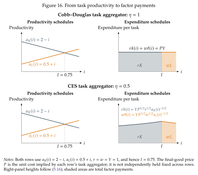
Figure 16 maps the productivity schedules on the left into these expenditure schedules on the right. Their heights depend on productivity, factor prices, output, and the final-good price \(P\), which equals unit cost. The blue area sums \(rk(i)\) over machine tasks and is therefore \(rK\); the orange area sums \(w\ell(i)\) over human tasks and is \(wL\). Dividing either area by the total area \(PY\) gives its factor share.

When \(\eta=1\), the productivity powers vanish and both expenditure schedules have the same height \(PY\). Area shares then equal lengths: \(\alpha_K=I\) and \(\alpha_L=1-I\). For \(\eta\neq1\), task lengths alone do not determine the expenditure shares. In the \(\eta=1/2\) example, tasks with lower productivity have higher expenditure per unit of task length because they are costly and hard to substitute away from. For \(\eta>1\), the productivity exponent is positive and the direction reverses.

Multiplying input demands by their prices gives input shares:

\[\begin{equation} \alpha_K\;\equiv\;\frac{rK}{PY} \;=\;\left(\frac rP\right)^{1-\eta}H_K(I),\qquad \alpha_L\;\equiv\;\frac{wL}{PY} \;=\;\left(\frac wP\right)^{1-\eta}H_L(I). \tag{5.17} \end{equation}\]

When \(\eta=1\) we aggregate with a Cobb-Douglas technology and optimality conditions give

\[\begin{equation} rk(i)=PY\quad(i<I),\qquad wn(i)=PY\quad(i>I). \tag{5.18} \end{equation}\]

Every equal-length task interval then receives the same input payment. Integrating gives the special result \(\alpha_K=I\) and \(\alpha_L=1-I\).