Part 2 / Section 5: Task-Based Model of Production Section 5.5

Comparative statics of task assignment

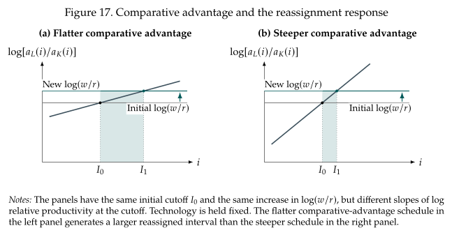
We can now look at how the firm's cost-minimizing choices respond to the relative input price \(w/r\). This response is summarized by the change in the assignment cutoff \(I\), which satisfies \(a_L(I)/a_K(I)=w/r\). Figure 17 shows what determines the size of this response. A fall in \(r\), with \(w\) fixed, raises the horizontal \(\log(w/r)\) line by the same amount in both panels. When log relative productivity changes slowly across nearby tasks, the new intersection is much farther to the right. Many tasks are close substitutes in who can perform them cheaply, so many change hands. A steep schedule instead means sharp differences in comparative advantage, and few tasks switch. The shaded widths measure the change in the assignment cutoff.

Taking logs and differentiating gives

\[\begin{equation} \left[\frac{a_L'(I)}{a_L(I)}-\frac{a_K'(I)}{a_K(I)}\right]\dd I \;=\;\dd\log(w/r) \quad\longrightarrow\quad \frac{\dd I}{\dd\log(w/r)} \;=\;\frac{1}{\dfrac{a_L'(I)}{a_L(I)}-\dfrac{a_K'(I)}{a_K(I)}}\;>\;0. \tag{5.19} \end{equation}\]

The denominator is positive because labor's relative productivity increases with the task index. A higher wage relative to the rental rate therefore expands the machine bundle and contracts the human bundle. The response is larger when comparative advantage changes less sharply around the cutoff.

We can also express this result using the elasticity of each productivity schedule with respect to the task index:

\[\begin{equation} \varepsilon_j(i)\;\equiv\;\frac{\dd\log a_j(i)}{\dd\log i} \;=\;\frac{i\,a_j'(i)}{a_j(i)},\qquad j\in\{K,L\}, \qquad \frac{\dd\log I}{\dd\log(w/r)} \;=\;\frac{1}{\varepsilon_L(I)-\varepsilon_K(I)}. \tag{5.20} \end{equation}\]

Under our assumptions, \(\varepsilon_L(I)>0\) and \(\varepsilon_K(I)<0\), so the gap in these elasticities is positive.

This result is particularly useful to characterize how the aggregate demand for capital and labor reacts to changes in prices.

How does reassignment affect substitution between the aggregate inputs?

Dividing the input demands in (5.15) cancels their common output and price terms:

\[\begin{equation} \frac{K}{L}\;=\;\left(\frac{w}{r}\right)^\eta\frac{H_K(I)}{H_L(I)}. \tag{5.21} \end{equation}\]

The limits of integration imply \(H_K'(I)=a_K(I)^{\eta-1}\) and \(H_L'(I)=-a_L(I)^{\eta-1}\). We use this to get the elasticity of substitution with task assignment:

\[\begin{align} \sigma\;\equiv\;\frac{\dd\log(K/L)}{\dd\log(w/r)} &\;=\;\underbrace{\eta}_{\text{fixed assignment}} \;+\;\underbrace{\left[ \frac{a_K(I)^{\eta-1}}{H_K(I)} +\frac{a_L(I)^{\eta-1}}{H_L(I)} \right]\frac{\dd I}{\dd\log(w/r)}}_{\text{task reassignment}}, \tag{5.22}\\ &\;=\;\eta+ \frac{I}{\varepsilon_L(I)-\varepsilon_K(I)} \left[\frac{a_K(I)^{\eta-1}}{H_K(I)} +\frac{a_L(I)^{\eta-1}}{H_L(I)}\right]\;>\;\eta. \nonumber \end{align}\]

At a fixed assignment, the firm substitutes between the quantities of machine-produced and human-produced tasks with elasticity \(\eta\). Allowing assignment to change adds a positive response: capital takes over marginal tasks previously performed by labor. Thus aggregate inputs are more substitutable than tasks at an interior cutoff, although \(\sigma\) need not be constant or exceed one when \(\eta<1\).

For example, with Cobb--Douglas task aggregation, \(\eta=1\), we have \(H_K(I)=I\) and \(H_L(I)=1-I\), so

\[\begin{equation} \sigma\;=\;1+\frac{1}{(1-I)}\frac{\dd \log I}{\dd\log(w/r)}. \tag{5.23} \end{equation}\]

The productivity schedules in Section 6.1, after relabeling its two labor inputs as capital and labor, imply \(\dd \log I/\dd\log(w/r)=\kappa (1-I)\) and hence \(\sigma=1+\kappa\). Section 6.2 instead shows how reassignment can raise an across-task elasticity \(\eta<1\) to an aggregate elasticity of exactly one.

The same reasoning applies to study changes in technology. Write task productivity as

\[\begin{equation} a_K(i)=\overline{a}_K\alpha_K(i),\qquad a_L(i)=\overline{a}_L\alpha_L(i), \tag{5.24} \end{equation}\]

where \(\overline{a}_K,\overline{a}_L>0\) scale productivity across all tasks and the fixed schedules \(\alpha_K(i),\alpha_L(i)\) describe its task-specific pattern. The cutoff condition becomes

\[\begin{equation} \frac{\alpha_L(I)}{\alpha_K(I)} \;=\;\frac{w}{r}\frac{\overline{a}_K}{\overline{a}_L} \quad\longrightarrow\quad \big[\varepsilon_L(I)-\varepsilon_K(I)\big]\dd\log I \;=\;\dd\log(w/r)+\dd\log(\overline{a}_K/\overline{a}_L). \tag{5.25} \end{equation}\]

Multiplying a productivity schedule by a constant does not change its elasticity with respect to the task index, so the same \(\varepsilon_j(I)\) apply. Holding \(w/r\) fixed therefore gives

\[\begin{equation} \left.\frac{\dd\log I}{\dd\log(\overline{a}_K/\overline{a}_L)}\right|_{w/r} \;=\;\frac{1}{\varepsilon_L(I)-\varepsilon_K(I)}\;>\;0. \tag{5.26} \end{equation}\]

An increase in \(\overline{a}_K\) lowers capital's cost of performing every task and expands the machine bundle. An increase in \(\overline{a}_L\) has the opposite effect. For assignment, a proportional increase in \(\overline{a}_K/\overline{a}_L\) has the same effect as the same proportional increase in \(w/r\).

Cheaper machines versus more productive machines

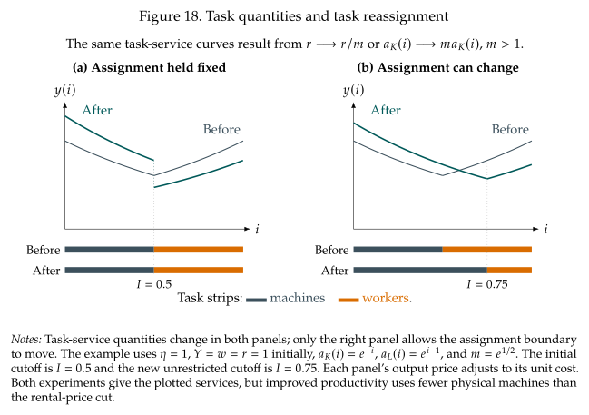
Figure 18 separates changing task quantities from changing who performs the tasks. First lower the rental price from \(r\) to \(r/m\), where \(m>1\), holding \(w\), technology, and final output fixed. Even if assignment is frozen, the firm changes the relative quantities of machine-produced and human-produced services. Allowing assignment to adjust also transfers a band of tasks from labor to capital, adding the reassignment response in (5.22).

Now compare this with keeping \(r\) fixed and multiplying the entire capital-productivity schedule by the same \(m\). At every task, the two experiments give the same machine unit cost:

\[\begin{equation} \frac{r/m}{a_K(i)}=\frac{r}{m a_K(i)}. \tag{5.27} \end{equation}\]

Consequently, they give the same assignment, task-service quantities, final-good unit cost, and labor use at the same output target. But they do not give the same physical capital use: producing each machine task service with the better technology requires \(1/m\) as much capital as producing it with the cheaper rental price. In terms of local responses to \(m\),

\[\begin{equation} \left.\frac{\dd\log(K/L)}{\dd\log m}\right|_{r\,\mapsto\,r/m}=\sigma, \qquad \left.\frac{\dd\log(K/L)}{\dd\log m}\right|_{a_K\,\mapsto\,m a_K}=\sigma-1. \tag{5.28} \end{equation}\]

The fixed-assignment components are respectively \(\eta\) and \(\eta-1\); the additional reassignment component is the same in both experiments. This is why equivalent improvements in the cost of machine services need not have the same effect on the number of machines used.