Part 1 / Section 4: Examples and Applications of the CES Production Function Section 4.2

Substitution and the scale of production

If capital becomes cheaper, the firm chooses a higher \(K/L\). Does this mean that it employs fewer workers? A higher ratio tells us about the input mix, but labor demand also depends on how much the firm produces as in our analysis under the Cobb-Douglas production function.

Consider a competitive industry with the technology in (3.1) and market demand for its final good

\[\begin{equation} Y=Bp^{-\varepsilon},\qquad B>0,\quad\varepsilon>0. \tag{4.8} \end{equation}\]

Here \(p\) is the final-good price and \(\varepsilon\) is the price elasticity of market demand in absolute value. We hold \(w\), technology, and demand parameters fixed and lower \(r\). Inputs are available to this industry at the given factor prices, so employment can adjust.

Constant returns and perfect competition imply \(p=c(r,w)\), the unit cost of production. So, the effect on demand depends on how much costs decrease when \(r\) goes down. The cost-minimization conditions are \(r=cF_K\) and \(w=cF_L\). Substituting the CES marginal products and solving for inputs per unit of output gives

\[\begin{align} \frac{K}{Y} &=z^{\sigma-1}\alpha^\sigma A_K^{\sigma-1} \left(\frac{c}{r}\right)^\sigma, & \frac{L}{Y} &=z^{\sigma-1}(1-\alpha)^\sigma A_L^{\sigma-1} \left(\frac{c}{w}\right)^\sigma. \tag{4.9} \end{align}\]

Constant-return to scale imply \(\,c\,=\,rK/Y\,+\,wL/Y\). So, we can substitute the input-to-output ratios from the cost minimization conditions to get

\[\begin{equation} c\;=\;z^{\sigma-1}c^\sigma \left[\alpha^\sigma\left(\frac{r}{A_K}\right)^{1-\sigma} +(1-\alpha)^\sigma\left(\frac{w}{A_L}\right)^{1-\sigma}\right]. \tag{4.10} \end{equation}\]

Dividing by \(c^\sigma\) and raising both sides to the power \(\frac{1}{1-\sigma}\) gives

\[\begin{equation} c(r,w)=\frac{1}{z} \left[\alpha^\sigma\left(\frac{r}{A_K}\right)^{1-\sigma} +(1-\alpha)^\sigma\left(\frac{w}{A_L}\right)^{1-\sigma} \right]^{\frac{1}{1-\sigma}}. \tag{4.11} \end{equation}\]

Taking logs and differentiating with respect to \(\log r\), we obtain

\[\begin{equation} \frac{\partial\log c}{\partial\log r} =\frac{\alpha^\sigma(r/A_K)^{1-\sigma}} {\alpha^\sigma(r/A_K)^{1-\sigma}+(1-\alpha)^\sigma(w/A_L)^{1-\sigma}} =\alpha_K. \tag{4.12} \end{equation}\]

The capital cost share therefore measures the sensitivity of unit cost to the rental price. Unlike Cobb--Douglas, this share changes with factor prices; the expression gives the elasticity at the current input mix.

Since \(p=c\), final-good demand implies

\[\begin{equation} \log Y=\log B-\varepsilon\log c \quad\longrightarrow\quad \frac{\partial\log Y}{\partial\log r}=-\varepsilon\alpha_K. \tag{4.13} \end{equation}\]

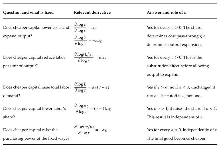
A one-percent fall in \(r\) lowers the output price by approximately \(\alpha_K\) percent and expands output by \(\varepsilon\alpha_K\) percent. Demand elasticity determines how strongly buyers respond to the lower price.

Does the expansion outweigh substitution away from labor?

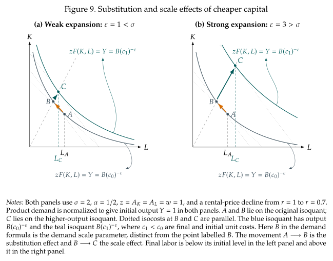
Figure 9 separates the two adjustments before we do the algebra. At \(A\), the firm uses the original cost-minimizing bundle. When \(r\) falls, the isocost becomes steeper and the fixed-output optimum moves to \(B\): the firm substitutes capital for labor along the original isoquant. Lower unit cost also reduces the output price and increases sales. Production then expands from \(B\) to \(C\) along the new constant-\(K/L\) ray, increasing both inputs. With weak product-demand response, this expansion does not restore the original employment level; with strong response, it more than restores it.

The connection to consumer theory

The movement from \(A\) to \(B\) is analogous to a compensated substitution effect: we change relative prices while holding the objective level fixed---output here, utility in consumer theory. The movement from \(B\) to \(C\) resembles the income effect geometrically because it moves to a higher isoquant along an expansion path. But its cause is different: the firm has no fixed income budget whose purchasing power has risen. Instead, lower production costs reduce the competitive output price and consumers buy more. The size of this scale effect depends on the elasticity of product demand \(\varepsilon\). Under constant returns, expanding output at the new factor prices scales both inputs proportionally, leaving \(K/L\) unchanged between \(B\) and \(C\). The comparison of \(\varepsilon\) with \(\sigma\) tells us which movement dominates employment.

Taking logs of (4.9) separates the amount produced from the labor required per unit:

\[\begin{equation} \log L=\log Y+(\sigma-1)\log z+\sigma\log(1-\alpha) +(\sigma-1)\log A_L+\sigma\log c-\sigma\log w. \tag{4.14} \end{equation}\]

The response of labor has two components:

\[\begin{equation} \frac{\partial\log L}{\partial\log r} \;=\; \left.\frac{\partial\log L}{\partial\log r}\right|_Y + \frac{\partial\log L}{\partial\log Y}\frac{\partial\log Y}{\partial\log r} \;=\;\underbrace{\sigma\alpha_K}_{\text{substitution}} -\underbrace{\varepsilon\alpha_K}_{\text{scale}} \;=\;\alpha_K(\sigma-\varepsilon). \tag{4.15} \end{equation}\]

Remember that a fall in \(r\) is a negative change in \(\log r\). Labor demand therefore rises if \(\varepsilon>\sigma\), falls if \(\varepsilon<\sigma\), and is unchanged if \(\varepsilon=\sigma\). In the Cobb--Douglas limit, \(\sigma=1\) and \(\alpha_K=\alpha\), recovering \(\alpha(1-\varepsilon)\) in (2.18).

Because \(w\) is fixed, \(\dd\log(w/r)=-\dd\log r\). We can also write

\[\begin{equation} \frac{\partial\log L}{\partial\log(w/r)} \;=\;\alpha_K(\varepsilon-\sigma), \qquad \frac{\partial\log(K/L)}{\partial\log(w/r)}\;=\;\sigma. \tag{4.16} \end{equation}\]

The capital--labor ratio rises as capital becomes cheaper even when total labor demand rises. When \(\sigma>1\), capital and labor are sufficiently substitutable that cheaper capital also lowers labor's cost share, as shown earlier.

A falling labor share and rising employment can therefore occur together:
Output expands enough to require more workers despite using less labor per unit of output.

Which outcomes depend on the scale of production?

At given factor prices and technology, neither factor shares nor prices depend on \(\varepsilon\). The input prices \(r\) and \(w\) are given, and the output price \(p=c(r,w)\) is determined by technology and input prices. Expanding production scales both input demands proportionally, so it does not change their cost shares. Differentiating the share expressions above, with \(w\) and technology fixed, gives

\[\begin{align} \dd\log\alpha_L&=\;(\sigma-1)\alpha_K\,\dd\log r, & \dd\log\alpha_K&=\;-(\sigma-1)\alpha_L\,\dd\log r. \tag{4.17} \end{align}\]

Neither response contains \(\varepsilon\). For \(\sigma>1\), cheaper capital lowers labor's share and raises capital's share, whatever the elasticity of final-good demand.

The real wage measured in units of this final good is \(w/p\). Since the nominal wage is fixed and \(p=c(r,w)\),

\[\begin{equation} \dd\log(w/p)=-\dd\log c=-\alpha_K\,\dd\log r. \tag{4.18} \end{equation}\]

Cheaper capital therefore raises this real wage, also independently of \(\varepsilon\). This measures purchasing power over the industry's good.

Taking Stock

Hold \(w\) and technology fixed, let \(r\) change, and use competitive pricing \(p=c(r,w)\) with final-good demand \(Y=Bp^{-\varepsilon}\), \(\varepsilon>0\). Input quantities and output can adjust. The table separates the change in labor per unit of output from the change in total employment and shows which outcomes depend on the demand elasticity.